Kernel Density Estimation

Authors:

Marc Steiner; Jonas Eschle

An introduction to Kernel Density Estimations, explanations to all methods implemented in zfit and a throughout comparison of the performance can be found in Performance of univariate kernel density estimation methods in TensorFlow by Marc Steiner from which many parts here are taken.

Estimating the density of a population can be done in a non-parametric manner. The simplest form is to create a density histogram, which is notably not so precise.

A more sophisticated non-parametric method is the kernel density estimation (KDE), which can be looked at as a sort of generalized histogram. In a kernel density estimation each data point is substituted with a so called kernel function that specifies how much it influences its neighboring regions. This kernel functions can then be summed up to get an estimate of the probability density distribution, quite similarly as summing up data points inside bins.

However, since the kernel functions are centered on the data points directly, KDE circumvents the problem of arbitrary bin positioning. Since KDE still depends on kernel bandwidth (a measure of the spread of the kernel function) instead of bin width, one might argue that this is not a major improvement. Upon closer inspection, one finds that the underlying PDF does depend less strongly on the kernel bandwidth than histograms do on bin width and it is much easier to specify rules for an approximately optimal kernel bandwidth than it is to do so for bin width.

Given a set of \(n\) sample points \(x_k\) (\(k = 1,\cdots,n\)), an exact kernel density estimation \(\widehat{f}_h(x)\) can be calculated as

(1)\[\widehat{f}_h(x) = \frac{1}{nh} \sum_{k=1}^n K\Big(\frac{x-x_k}{h}\Big)\]

where \(K(x)\) is called the kernel function, \(h\) is the bandwidth of the kernel and \(x\) is the value for which the estimate is calculated. The kernel function defines the shape and size of influence of a single data point over the estimation, whereas the bandwidth defines the range of influence. Most typically a simple Gaussian distribution (\(K(x) :=\frac{1}{\sqrt{2\pi}}e^{-\frac{1}{2}x^2}\)) is used as kernel function. The larger the bandwidth parameter :math:h the larger is the range of influence of a single data point on the estimated distribution.

Exact KDEs

Summary An exact KDE calculates the true sum of the kernels around the input points without approximating the dataset, leaving possibilities for the choice of a bandwidth. The computational complexity – especially the peak memory consumption – is proportional to the sample size. Therefore, this kind of PDF is better used for smaller datasets and a Grid KDE is preferred for larger data.

Explanation

Exact KDEs implement exactly Eq. (1) without any approximation and therefore no loss of information.

The computational complexity of the exact KDE above is given by \(\mathcal{O}(nm)\) where \(n\) is the number of sample points to estimate from and \(m\) is the number of evaluation points (the points where you want to calculate the estimate).

Due to this cost, the method is most often used for smaller datasamples.

There exist several approximative methods to decrease this complexity and therefore decrease the runtime as well.

Implementation

In zfit, the exact KDE KDE1DimExact takes an arbitrary kernel, which is a TensorFlow-Probability distribution.

import os
os.environ["ZFIT_DISABLE_TF_WARNINGS"] = "1"

import zfit
from zfit import z
import numpy as np
import matplotlib.pyplot as plt

obs = zfit.Space('x', (-5, 5))
gauss = zfit.pdf.Gauss(obs=obs, mu=0, sigma=2)
data = gauss.sample(1000)

kde = zfit.pdf.KDE1DimExact(data,
                            # obs, bandwidth, kernel,
                            # padding, weights, name
                            )
x = np.linspace(-5, 5, 200)
plt.plot(x, kde.pdf(x), label='Exact KDE')
plt.plot(x, gauss.pdf(x), label='True PDF')
plt.legend()

<matplotlib.legend.Legend at 0x7f52b0da7920>

Run interactively

Grid KDEs

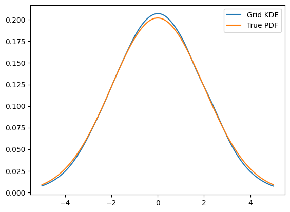
Summary To reduce the computational complexity, the input data can be finely binned into a histogram, where each bin serves as the sample point to a kernel. This is well suited for larger datasets. Like the exact KDE, this leaves the possibility to choose a bandwidth.

Explanation

The most straightforward way to decrease the computational complexity is by limiting the number of sample points. This can be done by a binning routine, where the values at a smaller number of regular grid points are estimated from the original larger number of sample points. Given a set of sample points \(X = \{x_0, x_1, ..., x_k, ..., x_{n-1}, x_n\}\) with weights :math:w_k and a set of equally spaced grid points \(G = \{g_0, g_1, ..., g_l, ..., g_{n-1}, g_N\}\) where \(N < n\) we can assign an estimate (or a count) \(c_l\) to each grid point \(g_l\) and use the newly found \(g_l\) to calculate the kernel density estimation instead.

(2)\[\widehat{f}_h(x) = \frac{1}{nh} \sum_{l=1}^N c_l \cdot K\Big(\frac{x-g_l}{h}\Big)\]

This lowers the computational complexity down to \(\mathcal{O}(N \cdot m)\). Depending on the number of grid points \(N\) there is tradeoff between accuracy and speed. However as we will see in the comparison chapter later as well, even for ten million sample points, a grid of size \(1024\) is enough to capture the true density with high accuracy. As described in the extensive overview by Artur Gramacki[@gramacki2018fft], simple binning or linear binning can be used, although the last is often preferred since it is more accurate and the difference in computational complexity is negligible.

Implementation

The implementation of Grid KDEs is similar to the exact KDEs, except that the former first bins the incomming data and uses this as a grid for the kernel. Therefore, it also takes parameters for the binning, such as the number of bins and the method.

data = gauss.sample(100_000)

kde = zfit.pdf.KDE1DimGrid(data,
                           # obs, bandwidth, kernel, num_grid_points,
                           # binning_method, padding, weights, name
                           )
plt.plot(x, kde.pdf(x), label='Grid KDE')
plt.plot(x, gauss.pdf(x), label='True PDF')
plt.legend()

<matplotlib.legend.Legend at 0x7f52b0e61640>

Bandwidth

Summary Bandwidth denotes the width of the kernel and aims usually at reducing the integrated squared error. There are two main distinction, a global and local bandwidths. The former is the same width for all kernels while the latter uses different bandwidth for each kernel and therefore can, in general, better reflect the local density, often at a computational cost.

Explanation

The optimal bandwidth is often defined as the one that minimizes the mean integrated squared error (\(MISE\)) between the kernel density estimation \(\widehat{f}_{h,norm}(x)\) and the true probability density function \(f(x)\), where \(\mathbb{E}_f\) denotes the expected value with respect to the sample which was used to calculate the KDE.

(3)\[MISE(h) = \mathbb{E}_f\int [\widehat{f}_{h,norm}(x) - f(x)]^2 dx\]

To find the optimal bandwidth it is useful to look at the second order derivative \(f^{(2)}\) of the unknown distribution as it indicates how many peaks the distribution has and how steep they are. For a distribution with many narrow peaks close together a smaller bandwidth leads to better result since the peaks do not get smeared together to a single peak for instance.

An asymptotically optimal bandwidth \(h_{AMISE}\) which minimizes a first-order asymptotic approximation of the \(MISE\) is then given by

(4)\[`h_{AMISE}(x) = \Big( \frac{1}{2N\sqrt{\pi} \| f^{(2)}(x)\|^2}\Big)^{\frac{1}{5}}`\]

where \(N\) is the number of sample points (or grid points if binning is used).

Implementation

zfit implements a few different bandwidth methods, of which not all are available for all KDEs.

Rule of thumb

Scott and Silvermann both proposed rule of thumb for the kernel bandwidth. These are approximate estimates that are a global parameter.

Adaptive methods

These methods calculate a local density parameter that is approximately \(/propto f( x ) ^ {-1/2}\), where \(f(x)\) is an initial estimate of the density. This can be calculated for example by using a rule of thumb to obtain an initial estimate. The main disadvantage is a higher computational complexity; the initial overhead as well as for the evaluation of the PDF. Most notably the memory consumption can be significantly higher.

FFT KDEs

Summary By rewriting the KDE as a discrete convolution and using the FFT, the density can be approximated interpolating between the discetized values.

Another technique to speed up the computation is rewriting the kernel density estimation as convolution operation between the kernel function and the grid counts (bin counts) calculated by the binning routine given above.

By using the fact that a convolution is just a multiplication in Fourier space and only evaluating the KDE at grid points one can reduce the computational complexity down to \(\mathcal{O}(\log{N} \cdot N)\)

Using Eq. (2) from above only evaluated at grid points gives us

(5)\[\widehat{f}_h(g_j) = \frac{1}{nh} \sum_{l=1}^N c_l \cdot K\Big(\frac{g_j-g_l}{h}\Big) = \frac{1}{nh} \sum_{l=1}^N k_{j-l} \cdot c_l\]

where \(k_{j-l} = K(\frac{g_j-g_l}{h})\).

If we set \(c_l = 0\) for all \(l\) not in the set \(\{1, ..., N\}\) and notice that \(K(-x) = K(x)\) we can extend Eq. (5) to a discrete convolution as follows

\[\widehat{f}_h(g_j) = \frac{1}{nh} \sum_{l=-N}^N k_{j-l} \cdot c_l = \vec{c} \ast \vec{k}\]

By using the convolution theorem we can fourier transform \(\vec{c}\) and \(\vec{k}\), multiply them and inverse fourier transform them again to get the result of the discrete convolution.

Due to the limitation of evaluating only at the grid points themselves, one needs to interpolate to get values for the estimated distribution at points in between.

Implementation

This is implemented in zfit as KDE1DimFFT. It supports similar arguments such as the grid KDEs except that the bandwidth can’t be variable.

kde = zfit.pdf.KDE1DimFFT(data,
                          # obs, bandwidth, kernel, num_grid_points, fft_method,
                          # binning_method, padding, weights, name
                          )
plt.plot(x, kde.pdf(x), label='FFT KDE')
plt.plot(x, gauss.pdf(x), label='True PDF')
plt.legend()

<matplotlib.legend.Legend at 0x7f52b0b76540>

ISJ KDEs

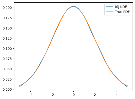
Summary A different take on KDEs is a new adaptive kernel density estimator based on linear diffusion processes. It performs especially well on data that do not follow a normal distribution. The method also includes an estimation for the optimal bandwidth.

The method is described completely in the paper ‘Kernel density estimation by diffusion’ by . The general idea is briefly sketched below.

As explained in Bandwidth, the optimal bandwidth is often defined as the one that minimizes the (\(MISE\)) as defined in Eq. (3) respectively a first-order asymptotic approximation \(h_{AMISE}\) as defined in Eq. (4).

As Sheather and Jones showed, this second order derivative can be estimated, starting from an even higher order derivative \(\|f^{(l+2)}\|^2\) by using the fact that \(\|f^{(j)}\|^2 = (-1)^j \mathbb{E}_f[f^{(2j)}(X)], \text{ } j\geq 1\)

\[h_j=\left(\frac{1+1 / 2^{j+1 / 2}}{3} \frac{1 \times 3 \times 5 \times \cdots \times(2 j-1)}{N \sqrt{\pi / 2}\left\|f^{(j+1)}\right\|^{2}}\right)^{1 /(3+2 j)} = \gamma_j(h_{j+1})\]

where \(h_j\) is the optimal bandwidth for the \(j\)-th derivative of \(f\) and the function \(\gamma_j\) defines the dependency of \(h_j\) on \(h_{j+1}\)

Their proposed plug-in method works as follows:

1. Compute \(\|\widehat{f}^{(l+2)}\|^2\) by assuming that \(f\) is the normal pdf with mean and variance estimated from the sample data

2. Using \(\|\widehat{f}^{(l+2)}\|^2\) compute \(h_{l+1}\)

3. Using \(h_{l+1}\) compute \(\|\widehat{f}^{(l+1)}\|^2\)

4. Repeat steps 2 and 3 to compute \(h^{l}\), \(\|\widehat{f}^{(l)}\|^2\), \(h^{l-1}\), \(\cdots\) and so on until \(\|\widehat{f}^{(2)}\|^2\) is calculated

5. Use \(\|\widehat{f}^{(2)}\|^2\) to compute \(h_{AMISE}\)

The weakest point of this procedure is the assumption that the true distribution is a Gaussian density function in order to compute \(\|\widehat{f}^{(l+2)}\|^2\). This can lead to arbitrarily bad estimates of \(h_{AMISE}\), when the true distribution is far from being normal.

Therefore Botev et al. took this idea further. Given the function \(\gamma^{[k]}\) such that

\[\gamma^{[k]}(h)=\underbrace{\gamma_{1}\left(\cdots \gamma_{k-1}\left(\gamma_{k}\right.\right.}_{k \text { times }}(h)) \cdots)\]

\(h_{AMISE}\) can be calculated as

\[h_{AMISE} = h_{1}=\gamma^{[1]}(h_{2})= \gamma^{[2]}(h_{3})=\cdots=\gamma^{[l]}(h_{l+1})\]

By setting \(h_{AMISE}=h_{l+1}\) and using fixed point iteration to solve the equation

\[h_{AMISE} = \gamma^{[l]}(h_{AMISE})\]

the optimal bandwidth \(h_{AMISE}\) can be found directly.

This eliminates the need to assume normally distributed data for the initial estimate and leads to improved accuracy, especially for density distributions that are far from normal. According to their paper increasing \(l\) beyond \(l=5\) does not increase the accuracy in any practically meaningful way. The computation is especially efficient if \(\gamma^{[5]}\) is computed using the Discrete Cosine Transform - an FFT related transformation.

The optimal bandwidth \(h_{AMISE}\) can then either be used for other kernel density estimation methods (like the FFT-approach discussed above) or also to compute the kernel density estimation directly using another Discrete Cosine Transform.

kde = zfit.pdf.KDE1DimISJ(data,
                          # obs, num_grid_points, binning_method,
                          # padding, weights, name
                          )
plt.plot(x, kde.pdf(x), label='ISJ KDE')
plt.plot(x, gauss.pdf(x), label='True PDF')
plt.legend()

<matplotlib.legend.Legend at 0x7f52b0cb8590>

Boundary bias and padding

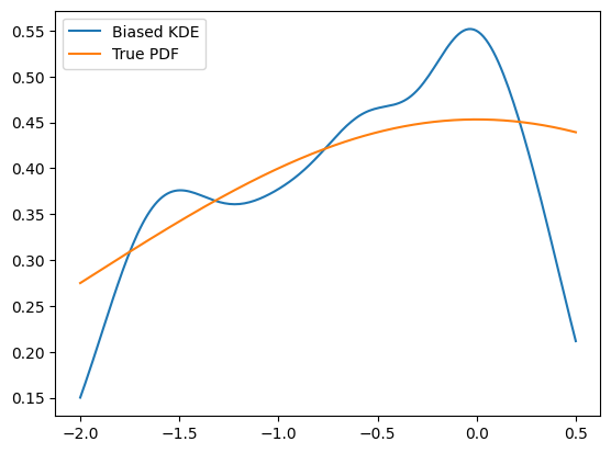
KDEs have a peculiar weakness: the boundaries, as the outside has a zero density. This makes the KDE go down at the bountary as well, as the density approaches zero, no matter what the density inside the boundary was.

obs = zfit.Space('x', (-2, 0.5))  # will cut of data at -2, 0.5
data_narrow = gauss.sample(1000, limits=obs)

kde = zfit.pdf.KDE1DimExact(data_narrow)

x = np.linspace(-2, 0.5, 200)
plt.plot(x, kde.pdf(x), label='Biased KDE')
plt.plot(x, gauss.pdf(x, obs), label='True PDF')
plt.legend()

<matplotlib.legend.Legend at 0x7f52b0ce3020>

There are two ways to circumvent this problem:

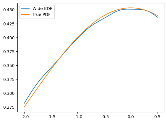
The best solution: providing a larger dataset than the default space the PDF is used in

obs_wide = zfit.Space('x', (-5, 5))
data_wide = gauss.sample(1000, limits=obs_wide)

kde = zfit.pdf.KDE1DimExact(data, obs=obs)

plt.plot(x, kde.pdf(x), label='Wide KDE')
plt.plot(x, gauss.pdf(x, obs), label='True PDF')
plt.legend()

<matplotlib.legend.Legend at 0x7f52b0ac3ef0>

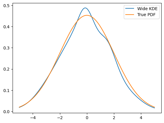
To get an idea of what happened, this is actually the full PDF. Notice that it is normalized over obs.

x = np.linspace(-5, 5, 200)
plt.plot(x, kde.pdf(x), label='Wide KDE')
plt.plot(x, gauss.pdf(x, obs), label='True PDF')
plt.legend()
x = np.linspace(-2, 0.5, 200)

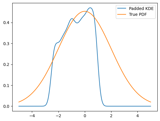
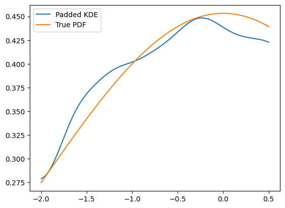
Another technique, as we may don’t have more data on the edges, is to mirror the existing data at the boundaries, which is equivalent to a boundary condition with a zero derivative. This is a padding technique and can improve the boundaries.

kde = zfit.pdf.KDE1DimExact(data_narrow, obs=obs, padding=0.2)

plt.plot(x, kde.pdf(x), label='Padded KDE')
plt.plot(x, gauss.pdf(x, obs), label='True PDF')
plt.legend()

<matplotlib.legend.Legend at 0x7f52b08a96d0>

However, one important drawback of this method is to keep in mind that this will actually alter the PDF to look mirrored. Plotting the PDF in a larger range makes this clear.

x = np.linspace(-5, 5, 200)
plt.plot(x, kde.pdf(x), label='Padded KDE')
plt.plot(x, gauss.pdf(x, obs), label='True PDF')
plt.legend()

<matplotlib.legend.Legend at 0x7f52b0a24800>

Download this tutorial notebook, script