5 minutes to zfit#

The zfit library provides a simple model fitting and sampling framework for a broad list of applications. This section is designed to give an overview of the main concepts and features in the context of likelihood fits in a crash course manner. The simplest example is to generate, fit and plot a Gaussian distribution.

The first step is to import zfit and to verify that the installation has been done successfully:

import os
os.environ["ZFIT_DISABLE_TF_WARNINGS"] = "1"
import numpy as np

import tensorflow as tf
import zfit
from zfit import z  # math backend of zfit

Since we want to generate/fit a Gaussian within a given range, the domain of the PDF is defined by an observable space. This can be created using the Space class

obs = zfit.Space('x', -10, 10)

The best interpretation of the observable at this stage is that it defines the name and range of the observable axis.

Using this domain, we can now create a simple Gaussian PDF. The most common PDFs are already pre-defined within the pdf module, including a simple Gaussian. First, we have to define the parameters of the PDF and their limits using the Parameter class:

mu = zfit.Parameter("mu", 2.4, -1, 5)
sigma = zfit.Parameter("sigma", 1.3,  0, 5)

With these parameters we can instantiate the Gaussian PDF from the library

gauss = zfit.pdf.Gauss(obs=obs, mu=mu, sigma=sigma)

It is recommended to pass the arguments of the PDF as keyword arguments.

The next stage is to create a dataset to be fitted. There are several ways of producing this within the zfit framework (see the Data section). In this case, for simplicity we simply produce it using numpy and the Data.from_numpy method:

data_np = np.random.normal(0, 1, size=10000)
data = zfit.Data(data_np, obs=obs)

Now we have all the ingredients in order to perform a maximum likelihood fit. Conceptually this corresponds to three basic steps:

create a loss function, in our case a negative log-likelihood \(\log\mathcal{L}\);
instantiate our choice of minimiser;
and minimise the log-likelihood.

# Stage 1: create an unbinned likelihood with the given PDF and dataset
nll = zfit.loss.UnbinnedNLL(model=gauss, data=data)

# Stage 2: instantiate a minimiser (in this case a basic minuit minimizer)
minimizer = zfit.minimize.Minuit()

# Stage 3: minimise the given negative likelihood
result = minimizer.minimize(nll)

This corresponds to the most basic example where the negative likelihood is defined within the pre-determined observable range and all the parameters in the PDF are floated in the fit. It is often the case that we want to only vary a given set of parameters. In this case it is necessary to specify which are the parameters to be floated (so all the remaining ones are fixed to their initial values).

Also note that we can now do various things with the pdf such as plotting the fitting result with the model gaussian without extracting the loss minimizing parameters from result. This is possible because parameters are mutable. This means that the minimizer can directly manipulate the value of the floating parameter. So when you call the minimizer.minimize() method the value of mu changes during the optimisation. gauss.pdf() then uses this new value to calculate the pdf.

# Stage 3: minimise the given negative likelihood but floating only specific parameters (e.g. mu)
result2 = minimizer.minimize(nll, params=[mu])

It is important to highlight that conceptually zfit separates the minimisation of the loss function with respect to the error calculation, in order to give the freedom of calculating this error whenever needed and to allow the use of external error calculation packages.

In order to get an estimate for the errors, it is possible to call Hesse that will calculate the parameter uncertainties. This uses the inverse Hessian to approximate the minimum of the loss and returns a symmetric estimate. When using weighted datasets, this will automatically perform the asymptotic correction to the fit covariance matrix, returning corrected parameter uncertainties to the user. The correction applied is based on Equation 18 in this paper.

To call Hesse, do:

param_hesse = result.hesse()
print(param_hesse)

{<zfit.Parameter 'mu' floating=True value=-0.001642>: {'error': np.float64(0.00996652061000915), 'cl': 0.68268949}, <zfit.Parameter 'sigma' floating=True value=0.9966>: {'error': np.float64(0.0070476677959662), 'cl': 0.68268949}}

which will return a dictionary of the fit parameters as keys with error values for each one. The errors will also be added to the result object and show up when printing the result.

While the hessian approximation has many advantages, it may not hold well for certain loss functions, especially for asymmetric uncertainties. It is also possible to use a more CPU-intensive error calculating with the errors method. This has the advantage of taking into account all the correlations and can describe well a a loss minimum that is not well approximated by a quadratic function (it is however not valid in the case of weights and takes considerably longer). It estimates the lower and upper uncertainty independently. As an example, with the Minuit one can calculate the MINOS uncertainties with:

param_errors, _ = result.errors()

print(param_errors)

{<zfit.Parameter 'mu' floating=True value=-0.001642>: {'lower': -0.009936759905952441, 'upper': 0.009996480602737185, 'is_valid': True, 'upper_valid': True, 'lower_valid': True, 'at_lower_limit': False, 'at_upper_limit': False, 'nfcn': 12, 'original': <MError number=0 name='mu' lower=-0.009936759905952441 upper=0.009996480602737185 is_valid=True lower_valid=True upper_valid=True at_lower_limit=False at_upper_limit=False at_lower_max_fcn=False at_upper_max_fcn=False lower_new_min=False upper_new_min=False nfcn=12 min=-0.0016718538509566574>, 'cl': 0.68268949}, <zfit.Parameter 'sigma' floating=True value=0.9966>: {'lower': -0.0070398484849763885, 'upper': 0.0070548717864089006, 'is_valid': True, 'upper_valid': True, 'lower_valid': True, 'at_lower_limit': False, 'at_upper_limit': False, 'nfcn': 12, 'original': <MError number=1 name='sigma' lower=-0.0070398484849763885 upper=0.0070548717864089006 is_valid=True lower_valid=True upper_valid=True at_lower_limit=False at_upper_limit=False at_lower_max_fcn=False at_upper_max_fcn=False lower_new_min=False upper_new_min=False nfcn=12 min=0.9966461004335957>, 'cl': 0.68268949}}

Once we’ve performed the fit and obtained the corresponding uncertainties, it is now important to examine the fit results. The object result (FitResult) has all the relevant information we need:

print(f"Function minimum: {result.fmin}")
print(f"Converged: {result.converged}")
print(f"Valid: {result.valid}")

Function minimum: 14155.448640891282

Converged: True

Valid: True

This is all available if we print the fitresult (not shown here as display problems).

print(result)

Similarly one can obtain only the information on the fitted parameters with

# Information on all the parameters in the fit
print(result.params)

# Printing information on specific parameters, e.g. mu
print("mu={}".format(result.params[mu]['value']))

name      value  (rounded)        hesse               errors    at limit
------  ------------------  -----------  -------------------  ----------
mu             -0.00167185  +/-    0.01  - 0.0099   +   0.01       False


sigma             0.996646  +/-   0.007  -  0.007   + 0.0071       False

mu=-0.0016718538509566574

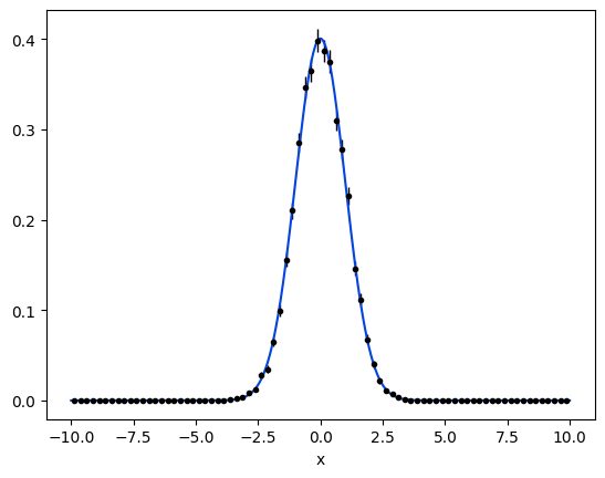
As already mentioned, there is no dedicated plotting feature within zfit. However, we can easily use external libraries, such as matplotlib and mplhep, a library for HEP-like plots , to do the job:

import mplhep
import matplotlib.pyplot as plt
import numpy as np

# plot the data as a histogramm
bins = 80
mplhep.histplot(data.to_binned(bins), yerr=True, density=True, color='black', histtype='errorbar')

# evaluate the func at multiple x and plot
x_plot = np.linspace(obs.v1.lower, obs.v1.upper, num=1000)
y_plot = gauss.pdf(x_plot)
plt.plot(x_plot, y_plot, color='xkcd:blue')
plt.show()

The full script can be downloaded here.