Bayesian Inference

Introduction

zfit provides a Bayesian inference framework that allows you to perform parameter estimation using MCMC (Markov Chain Monte Carlo) sampling. This functionality complements the frequentist approach of maximum likelihood estimation by incorporating prior knowledge and providing full posterior distributions for parameters.

Key Components

• Priors: Define prior distributions for parameters

• EmceeSampler: MCMC sampler based on the emcee ensemble sampler

• PosteriorSamples: Result object for analyzing posterior distributions

• ArviZ Integration: Advanced diagnostics and visualization through ArviZ

Priors

zfit provides several built-in prior distributions that can be attached to parameters:

import zfit
from zfit import prior

# Create parameters with priors
mu = zfit.Parameter("mu", 0.0, -5.0, 10.0, prior=prior.Normal(mu=0.0, sigma=2.0))
sigma = zfit.Parameter("sigma", 1.0, 0.1, 5.0, prior=prior.HalfNormal(sigma=2.0))
frac = zfit.Parameter("frac", 0.5, 0.0, 1.0, prior=prior.Uniform(lower=0.0, upper=1.0))

Available Prior Distributions

import zfit
from zfit import prior

# List all available prior distributions
available_priors = [name for name in dir(prior) if not name.startswith('_') and hasattr(getattr(prior, name), '__call__')]
print("Available prior distributions:")
for p in sorted(available_priors):
    print(f"  - {p}")

Available prior distributions:

  - AffineTransform

  - Beta

  - Cauchy

  - ConstraintType

  - Exponential

  - Gamma

  - HalfNormal

  - IdentityTransform

  - KDE

  - LogNormal

  - LogTransform

  - LowerBoundTransform

  - Normal

  - Poisson

  - PriorConstraint

  - SigmoidTransform

  - StudentT

  - Uniform

  - UpperBoundTransform

MCMC Sampling

We can sample from the posterior distribution using MCMC methods. zfit provides the EmceeSampler, which is based on the popular emcee library.

from zfit.mcmc import EmceeSampler

# Create sampler with custom settings
sampler = EmceeSampler(
    nwalkers=32,      # Number of walkers (default: 2 × n_params)
    verbosity=0,      # Verbosity level (0-6: no progress, 7: phases, 8+: progress bars)
)

print("EmceeSampler created with:")
print(f"  - nwalkers: {sampler.nwalkers}")

EmceeSampler created with:

  - nwalkers: 32

Basic Usage Example

Here’s a complete example of Bayesian inference with zfit:

import zfit
from zfit.mcmc import EmceeSampler
import numpy as np

# Set seed for reproducible results
zfit.settings.set_seed(42)

# Create parameters with priors
mu = zfit.Parameter("mu", 5.0, 4.5, 5.5,
                    prior=zfit.prior.Uniform(lower=4.8, upper=5.2))
sigma = zfit.Parameter("sigma", 0.1, 0.05, 0.3,
                      prior=zfit.prior.HalfNormal(sigma=0.1))

# Create a model
obs = zfit.Space("x", -10, 10)
gauss = zfit.pdf.Gauss(mu=mu, sigma=sigma, obs=obs)

# Create some data
data = zfit.Data.from_numpy(obs=obs, array=np.random.normal(5.0, 0.12, 1000))

# Create negative log-likelihood loss
nll = zfit.loss.UnbinnedNLL(model=gauss, data=data)

# Sample from the posterior (small sample for docs)
sampler = EmceeSampler(nwalkers=16, verbosity=0)
posterior = sampler.sample(nll, n_samples=100, n_warmup=50)

# Display results
print("Posterior sampling completed:")
print(f"  - Parameters: {posterior.param_names}")
print(f"  - Samples shape: {posterior.samples.shape}")
print(f"  - Total samples: {len(posterior.samples)} ({sampler.nwalkers} walkers × {100} steps)")

Posterior sampling completed:

  - Parameters: ['mu', 'sigma']

  - Samples shape: (1600, 2)

  - Total samples: 1600 (16 walkers × 100 steps)

Posterior Analysis

The PosteriorSamples object provides methods for analyzing the posterior:

# Get posterior statistics
mu_mean = posterior.mean("mu")
mu_std = posterior.std("mu")

print(f"Parameter 'mu':")
print(f"  - Mean: {mu_mean:.4f}")
print(f"  - Std:  {mu_std:.4f}")

# Get credible intervals
lower, upper = posterior.credible_interval("mu", alpha=0.05)  # 95% CI
print(f"  - 95% CI: [{lower:.4f}, {upper:.4f}]")

# Check convergence
print(f"\nConvergence:")
print(f"  - Converged: {posterior.converged}")
print(f"  - R̂: {posterior.rhat}")
print(f"  - ESS: {posterior.ess}")

Parameter 'mu':

  - Mean: 4.9967

  - Std:  0.0038

  - 95% CI: [4.9883, 5.0041]

Convergence:

  - Converged: True

  - R̂: [1.01587368 1.00995116]

  - ESS: [1899.44063636 1873.02121012]

Posterior Integration

The posterior samples integrate with zfit’s parameter system:

print("Original parameter values:")
print(f"  - mu: {mu.value():.4f}")
print(f"  - sigma: {sigma.value():.4f}")

# Set parameters to posterior means
posterior.update_params()

print("\nAfter updating with posterior means:")
print(f"  - mu: {mu.value():.4f}")
print(f"  - sigma: {sigma.value():.4f}")

Original parameter values:

  - mu: 5.0000

  - sigma: 0.1000

After updating with posterior means:

  - mu: 4.9967

  - sigma: 0.1187

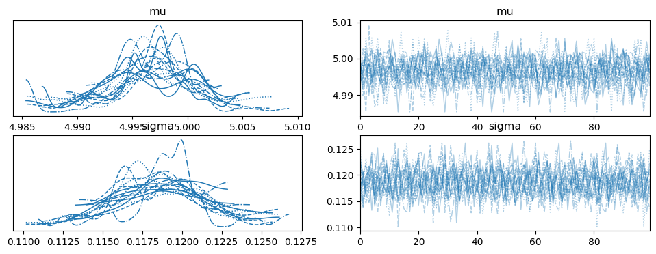
For more advanced usage, you can also use the ArviZ library to visualize and analyze the posterior distributions, including trace plots, pair plots, and more.

import arviz as az

# Convert posterior samples to ArviZ InferenceData
inference_data = posterior.to_arviz()

# Plot trace and pair plots
az.plot_trace(inference_data)
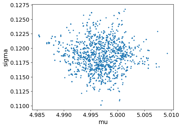
az.plot_pair(inference_data)

<Axes: xlabel='mu', ylabel='sigma'>

Make live