Upgrade guide to 0.20

With version 0.20, zfit prepares for a more stable and user-friendly interface. This guide will help you to upgrade your code to the new version and demonstrate the most significant changes. It is meant for people who are already familiar with zfit and want to upgrade their code.

Not all changes are everywhere reflected in the docs, help is highly appreciated!

from __future__ import annotations

import numpy as np
# standard imports
import zfit
import zfit.z.numpy as znp  # use this "numpy-like" for mathematical operations
from zfit import z

/home/docs/checkouts/readthedocs.org/user_builds/zfit/envs/0.20.1/lib/python3.12/site-packages/zfit/__init__.py:59: UserWarning: TensorFlow warnings are by default suppressed by zfit. In order to show them, set the environment variable ZFIT_DISABLE_TF_WARNINGS=0. In order to suppress the TensorFlow warnings AND this warning, set ZFIT_DISABLE_TF_WARNINGS=1.
  warnings.warn(

# example usage of the new numpy-like


@z.function
def maximum(x, y):
    return znp.maximum(x, y)

Parameters

The largest news comes from parameters: the NameAlreadyTakenError is gone (!). Multiple parameters with the same name can now be created and co-exist. The only limit is: they must not exist within the same PDF/loss etc., as this would lead to ambiguities.

param1 = zfit.Parameter("param1", 1, 0, 10)
param1too = zfit.Parameter("param1", 2, 0, 10)
# no error!

Labels

Many objects, including parameters, can now have a label. This label is purely human-readable and can be used for plotting, printing, etc. It can contain arbitrary characters.

The name of objects still exists and will in a future version probably be used for identification purpose (in conjunction with serialization). Therefore, use label for human-readable names and avoid name for that purpose.

param1again = zfit.Parameter("param1", 3, 0, 10, label=r"$param_1$ [GeV$^2$]")

Space

As explained in the github discussion thread there are major improvements and changes.

• multispaces (adding two spaces, having disjoint observables) are now deprecated and will be removed. The new TruncatedPDF supports multiple spaces as limits and achieves a similar, if not better, functionality.

• the return type of Space.limit will be changed in the future. For forwards compatibility, use Space.v1.limit (or similar methods) instead of Space.limit. The old one is still available via Space.v0.limit.

• new ways of creating spaces

obs1 = zfit.Space("obs1", -1, 1)  # no tuple needed anymore
obs2 = zfit.Space("obs2", lower=-1, upper=1, label="observable two")

# create a space with multiple observables
obs12 = obs1 * obs2

# limits are now as one would naively expect, and area has been renamed to volume (some are tensors, but that doesn't matter: they behave like numpy arrays)

# this allows, for example, for a more intuitive way
np.linspace(*obs12.v1.limits, 7)

array([[-1.        , -1.        ],
       [-0.66666667, -0.66666667],
       [-0.33333333, -0.33333333],
       [ 0.        ,  0.        ],
       [ 0.33333333,  0.33333333],
       [ 0.66666667,  0.66666667],
       [ 1.        ,  1.        ]])

Data

Data handling has been significantly simplified and streamlined.

• all places (or most) take directly numpy arrays, tensors or pandas DataFrame as input, using a Data object is not necessary anymore (but convenient, as it cuts the data to the space)

• Data objects can now be created without the specific constructors (e.g. zfit.Data.from_pandas), but directly with the data. The constructors are still available for convenience and for more options.

• Data objects are now stateless and offer instead with-methods to change the data. For example, with_obs, with_weights (can be None to have without weights) etc.

• The SamplerData has been overhauld and has now a more public API including a update_data method that allows to change the data without creating a new object and without relying on a create_sampler method from a PDF.

• zfit.data.concat has been added to concatenate data objects, similar to pd.concat.

data1_obs1 = zfit.Data(np.random.uniform(0, 1, 1000), obs=obs1)
data1_obs2 = zfit.Data(np.random.uniform(0, 1, 1000), obs=obs2, label="My favourite $x$")
data2_obs1 = zfit.Data(np.random.normal(0, 1, 1000), obs=obs1)

# similar like pd.concat
data_obs12 = zfit.data.concat([data1_obs1, data1_obs2], axis="columns")
data_obs1 = zfit.data.concat([data1_obs1, data2_obs1], axis="index")

# data can be accessed with "obs" directly

Binning

Using a binned space has now the effect of creating a binned version. This happens for Data and PDF objects.

obs1_binned = obs1.with_binning(12)
data_binned = zfit.Data(np.random.normal(0, 0.2, 1000), obs=obs1_binned)

PDFs

• there are a plethora of new PDFs, mostly covering physics inspired use-cases. Amongst the interesting ones are a GeneralizedCB, a more general version of the DoubleCB that should be preferred in the future. Also a Voigt profile is available, Bernstein polynomials, QGauss, GaussExpTail, etc.

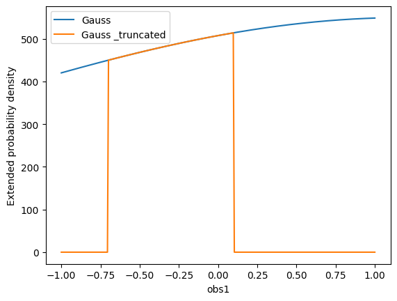
• the TruncatedPDF has been added to allow for a more flexible way of truncating a PDF. Any PDF can be converted to a truncated version using to_truncated (which, by default, truncates to the limits of the space).

• PDFs have a new plot method that allows for a quick plotting of the PDF (it takes an “obs” argument that allows to simply project it!). This is still experimental and may changes, the main purpose is to allow for a quick check of the PDF in interactive environments. The function is fully compatible with matplotlib and takes an ax argument, it also allows to pass through any keyword arguments to the plotting function.

# all the new PDFs

# create a PDF
pdf = zfit.pdf.Gauss(
    mu=zfit.Parameter("mu", 1.2), sigma=param1again, obs=obs1, extended=1000
)  # using an extended PDF, the truncated pdf automatically rescales
pdf.plot.plotpdf()  # quick plot
# truncate it
pdf_truncated = pdf.to_truncated(limits=(-0.7, 0.1))
pdf_truncated.plot.plotpdf()

/tmp/ipykernel_1447/1765407134.py:5: ExperimentalFeatureWarning: The function <function assert_initialized.<locals>.wrapper at 0x7fb5cd1789a0> is EXPERIMENTAL, potentially unstable and likely to change in the future! Use it with caution and feedback (Gitter, Mattermost, e-mail or https://github.com/zfit/zfit/issues) is very welcome!
  pdf.plot.plotpdf()  # quick plot

<Axes: xlabel='obs1', ylabel='Extended probability density'>

# binned pdfs from space work like the data
gauss_binned = zfit.pdf.Gauss(mu=zfit.Parameter("mu", 2.5), sigma=param1again, obs=obs1_binned, extended=1000)

/home/docs/checkouts/readthedocs.org/user_builds/zfit/envs/0.20.1/lib/python3.12/site-packages/zfit/models/tobinned.py:71: AdvancedFeatureWarning: Either you're using an advanced feature OR causing unwanted behavior. To turn this warning off, use `zfit.settings.advanced_warnings['extend_wrapped_extended'] = False`  or 'all' (use with care) with `zfit.settings.advanced_warnings['all'] = False
PDF Gauss Gauss is already extended, but extended also given 1000. Will use the given yield.
  warn_advanced_feature(

# as mentioned before, PDFs can be evaluated directly on numpy arrays or pandas DataFrames
pdf.pdf(data_obs1.to_pandas())

<tf.Tensor: shape=(1671,), dtype=float64, numpy=
array([0.50788917, 0.54627208, 0.51583184, ..., 0.54270569, 0.5349698 ,
       0.46742585])>

Loss and minimizer

They stay mostly the same (apart from improvements behind the scenes and bugfixes). Losses take now directly the data and the model, without the need of a Data object (if the data is already cut to the space).

To use the automatic gradient, set gradient="zfit" in the minimizer. This can speed up the minimization for larger fits.

Updated params

The minimizer currently updates the parameter default values after each minimization. To keep this behavior, add update_params() call after the minimization.

(experimentally, the update can be disabled with zfit.run.experimental_disable_param_update(True), this will probably be the default in the future. Pay attention that using this experimental features most likely breaks current scripts. Feedback on this new feature is highly welcome!)

loss = zfit.loss.ExtendedUnbinnedNLL(model=pdf, data=data2_obs1.to_pandas())
minimizer = zfit.minimize.Minuit(
    gradient="zfit"
)  # to use the automatic gradient -> can fail, but can speed up the minimization

result = minimizer.minimize(loss).update_params()
pdf.plot.plotpdf(full=False)  # plot only the pdf, no labels

<Axes: >

Result and serialization

The result stays similar but can now be pickled like any object in zfit! (this was not possible before, only after calling freeze on the result)

This works directly using dill (a library that extends pickle), but can fail if the garbage collector is not run. Therefore, zfit provides a slightly modified dill that can work as a drop-in replacement.

The objects can be saved and loaded again and used as before. Ideal to store the minimum of a fit and use it later for statistical treatments, plotting, etc.

result_serialized = zfit.dill.dumps(result)
result_deserialized = zfit.dill.loads(result_serialized)
result_deserialized.errors()

({<zfit.Parameter 'mu' floating=True value=-0.04361>: {'lower': -0.06589993126480596,
   'upper': 0.061929554967183005,
   'is_valid': True,
   'upper_valid': True,
   'lower_valid': True,
   'at_lower_limit': False,
   'at_upper_limit': False,
   'nfcn': 26,
   'original': ┌──────────┬───────────────────────┐
│          │          mu           │
├──────────┼───────────┬───────────┤
│  Error   │   -0.07   │   0.06    │
│  Valid   │   True    │   True    │
│ At Limit │   False   │   False   │
│ Max FCN  │   False   │   False   │
│ New Min  │   False   │   False   │
└──────────┴───────────┴───────────┘,
   'cl': 0.68268949},
  <zfit.Parameter 'param1' floating=True value=0.9233>: {'lower': -0.09306807713512023,
   'upper': 0.13195262544703426,
   'is_valid': True,
   'upper_valid': True,
   'lower_valid': True,
   'at_lower_limit': False,
   'at_upper_limit': False,
   'nfcn': 40,
   'original': ┌──────────┬───────────────────────┐
│          │        param1         │
├──────────┼───────────┬───────────┤
│  Error   │   -0.09   │   0.13    │
│  Valid   │   True    │   True    │
│ At Limit │   False   │   False   │
│ Max FCN  │   False   │   False   │
│ New Min  │   False   │   False   │
└──────────┴───────────┴───────────┘,
   'cl': 0.68268949}},
 None)

Parameters as arguments

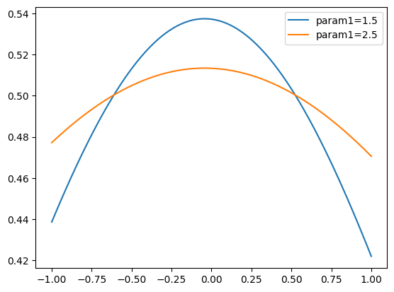
The values of the parameters can now be directly used as arguments in functions of PDFs/loss. Methods in the pdf also take the parameters as arguments.

The name of the argument has to match the name of the parameter given in initialization (or can also be the parameter itself).

from matplotlib import pyplot as plt

x = znp.linspace(*obs1.v1.limits, 1000)
plt.plot(x, pdf.pdf(x, params={"param1": 1.5}), label="param1=1.5")
plt.plot(x, pdf.pdf(x, params={param1again: 2.5}), label="param1=2.5")
plt.legend()

<matplotlib.legend.Legend at 0x7fb5c8480470>

import tqdm

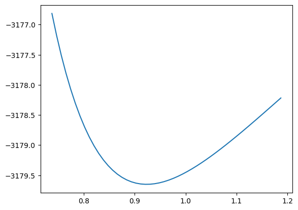
# similar for the loss
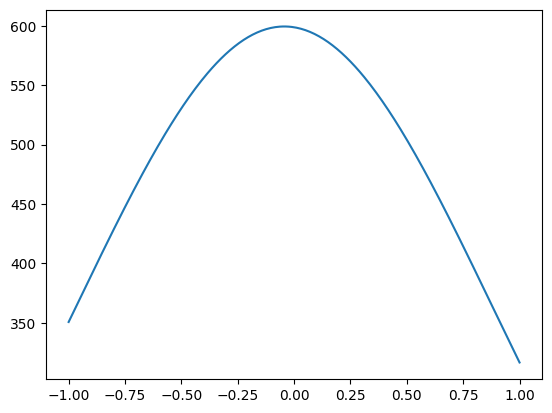
param1dict = result_deserialized.params[param1again]
param1min = param1dict["value"]
lower, upper = param1dict["errors"]["lower"], param1dict["errors"]["upper"]
x = np.linspace(param1min + 2 * lower, param1min + 2 * upper, 50)
y = []
param1again.floating = False  # not minimized
for x_i in tqdm.tqdm(x):
    param1again.set_value(x_i)
    minimizer.minimize(loss).update_params()  # set nuisance parameters to minimum
    y.append(loss.value())
plt.plot(x, y)

  0%|          | 0/50 [00:00<?, ?it/s]

  2%|▏         | 1/50 [00:00<00:28,  1.72it/s]

  6%|▌         | 3/50 [00:00<00:09,  4.76it/s]

 10%|█         | 5/50 [00:00<00:06,  7.00it/s]

 14%|█▍        | 7/50 [00:01<00:05,  8.59it/s]

 18%|█▊        | 9/50 [00:01<00:04,  9.76it/s]

 22%|██▏       | 11/50 [00:01<00:03, 10.61it/s]

 26%|██▌       | 13/50 [00:01<00:03, 11.20it/s]

 30%|███       | 15/50 [00:01<00:03, 11.64it/s]

 34%|███▍      | 17/50 [00:01<00:02, 11.91it/s]

 38%|███▊      | 19/50 [00:02<00:02, 12.13it/s]

 42%|████▏     | 21/50 [00:02<00:02, 12.27it/s]

 46%|████▌     | 23/50 [00:02<00:02, 12.39it/s]

 50%|█████     | 25/50 [00:02<00:02, 12.45it/s]

 54%|█████▍    | 27/50 [00:02<00:01, 12.52it/s]

 58%|█████▊    | 29/50 [00:02<00:01, 12.55it/s]

 62%|██████▏   | 31/50 [00:02<00:01, 12.58it/s]

 66%|██████▌   | 33/50 [00:03<00:01, 12.59it/s]

 70%|███████   | 35/50 [00:03<00:01, 12.61it/s]

 74%|███████▍  | 37/50 [00:03<00:01, 12.62it/s]

 78%|███████▊  | 39/50 [00:03<00:00, 12.62it/s]

 82%|████████▏ | 41/50 [00:03<00:00, 12.61it/s]

 86%|████████▌ | 43/50 [00:03<00:00, 12.63it/s]

 90%|█████████ | 45/50 [00:04<00:00, 12.64it/s]

 94%|█████████▍| 47/50 [00:04<00:00, 12.65it/s]

 98%|█████████▊| 49/50 [00:04<00:00, 12.63it/s]

100%|██████████| 50/50 [00:04<00:00, 11.19it/s]

[<matplotlib.lines.Line2D at 0x7fb5c8480e60>]

# creating a PDF looks also different, but here we use the name of the parametrization and the axis (integers)


class MyGauss2D(zfit.pdf.ZPDF):
    _PARAMS = ("mu", "sigma")
    _N_OBS = 2

    @zfit.supports()  # this allows the params magic
    def _unnormalized_pdf(self, x, params):
        x0 = x[0]  # this means "axis 0"
        x1 = x[1]  # this means "axis 1"
        mu = params["mu"]
        sigma = params["sigma"]
        return znp.exp(-0.5 * ((x0 - mu) / sigma) ** 2) * x1  # fake, just for demonstration

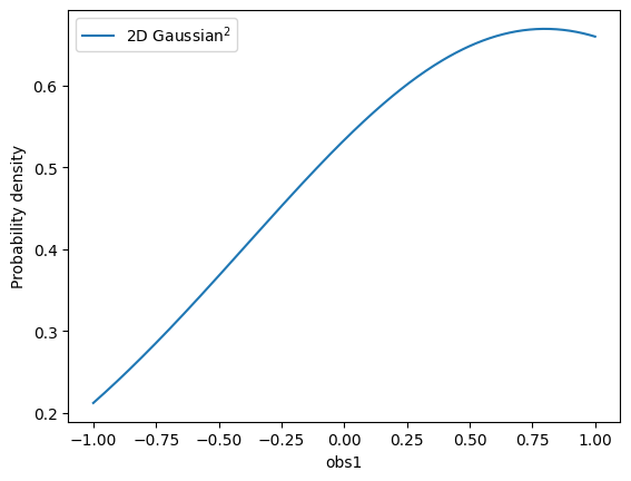
gauss2D = MyGauss2D(mu=0.8, sigma=param1again, obs=obs12, label="2D Gaussian$^2$")
gauss2D.plot.plotpdf(obs="obs1")  # we can project the 2D pdf to 1D

<Axes: xlabel='obs1', ylabel='Probability density'>